Mountains are fun! Here, check out this mountain on Google Maps:

The reason I'm showing you this is because you're going to make your own mountain with Python! 🐍🚀

Final demo and code

Getting started

We're going to be using Repl.it, a free, online code editor, to write our code. To get started, click here to visit the starter project. Once it loads, click the "Fork" button to start coding.

Once your fork loads, you should notice a blank file called main.py and a file called mountain.csv, which contains some data. If you see this, you're ready to move on to the next step!

We're going to use 3 libraries for this workshop: pandas, numpy, matplotlib, and mpl_toolkits.

Start by importing these libraries at the top of the main.py file:

import pandas as pd
import numpy as np
import matplotlib.pyplot as plt
from mpl_toolkits.mplot3d import Axes3D

• pandas allows importing and working with data from datasets. We're going to use it to manage our CSV file.
• numpy is a library that allows for easy scientific computing. We're going to use it to manage arrays in this workshop.
• matplotlib is a library for data visualization—histograms, scatter plots and bar graphs, etc. We're going to use it to make our mountain.
• The mpl_toolkits are collections of functions that extend the matplotlib application. This will enable us to plot in a 3D plane, rather than 2D.

Once you've imported these libraries, add a blank line, then add:

DataFrame = pd.read_csv('mountain.csv')

Here, we're creating a variable called DataFrame, which will use pandas to read the mountain.csv file.

Under that line, add:

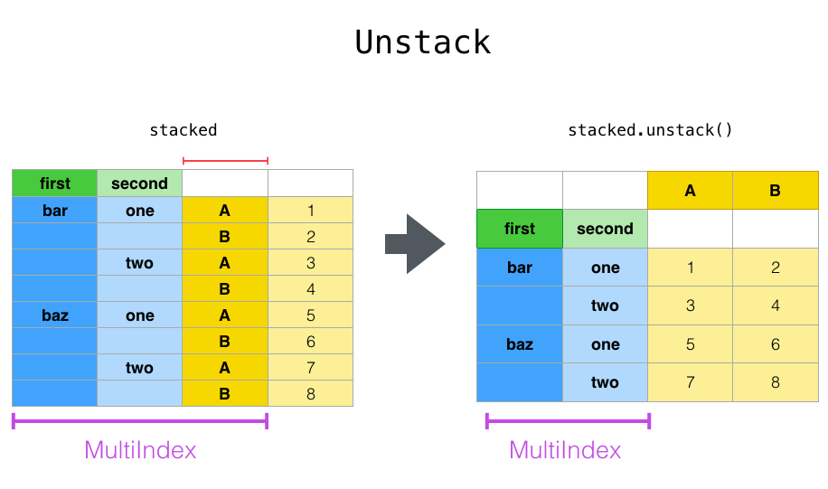
DataFrame = DataFrame.unstack()

The unstack() function unstacks the row to columns. Here's a diagram that shows how it works:

Under that, add:

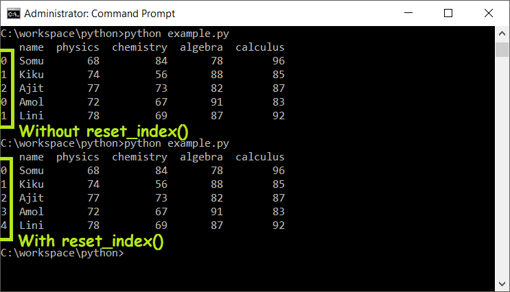
DataFrame = DataFrame.reset_index()

When you concatenate, sort, join or do some rearrangements with your DataFrame, the index gets shuffled or out of order. To reset the index of a DataFrame, we use reset_index() to resort the indexes.

Under that, add:

DataFrame.columns = ['X', 'Y', 'Z']

Your DataFrame contains three columns without labels, so we need to assign labels to the columns. DataFrame.columns assigns the first column to X, the second to Y, the third to Z. In our 3D graph, this will correspond to latitude, longitude, and altitude.

Fun fact: we have exactly 552 coordinates.

Under that, add:

DataFrame['X'] = pd.Categorical(DataFrame['X'])

Categorical is a pandas data type which is used to save memory space and speed up computation. you can convert using syntax pd.Categorical() with parameter DataFrame['X'].

Next, add:

DataFrame['X'] = DataFrame['X'].cat.codes

By using cat.codes, we get unique integer values for each value of X in an array in the position if the actual values, even if the value is none. Then, it returns a unique numeric value.

Suppose your data contains a column named "Birds" with 100 rows, which has only two types of values—parrot and owl—repeated in rows. Even though we only have two types of data, we have 100 rows of them so the computer will treat every value as unique. To save memory, we specify the similar set of values as a category, so that the computer doesn't allocate memory every time it encounters that value. Instead, it will just assign a reference to the value. If this sounds like gibberish to you, don't worry—all you need to know is that we're doing some fancy computer memory saving things.

Under this line, add:

fig = plt.figure(figsize=(6, 8))

Here, we're using plt.figure() to create a figure window and assigning it to a variable called fig.

Next, add:

ax = fig.gca(projection='3d')

fig.gca() with the argument projection=3d returns the three-dimensional axes associated with the figure window. This is stored in a variable called ax.

Next, add:

ax.plot_trisurf(DataFrame['X'], DataFrame['Y'], DataFrame['Z'], cmap=plt.cm.jet, linewidth=0.2)

This creates a three-dimensional plot.

• cmap defines the colormap of the plot. We're using the jet colormap. Learn more about the different types of colormaps here.
• linewidth=0.2 makes the curves smoother.

Next, add:

plt.title("Mount San Bruno")
plt.xlabel("x axis")
plt.ylabel("y axis")

• plt.title adds a title to the plot
• plot.xlabel and plot.ylabel add labels to the x and y-axis of the plot.

Next, let's display the plot!

plt.show()

plt.show opens an interactive window that displays your figure.

import pandas as pd

import numpy as np

import matplotlib.pyplot as plt

from mpl_toolkits.mplot3d import Axes3D

DataFrame = pd.read_csv('mountain.csv')

DataFrame = DataFrame.unstack()

DataFrame = DataFrame.reset_index()

DataFrame.columns = ['X', 'Y', 'Z']

DataFrame['X'] = pd.Categorical(DataFrame['X'])

DataFrame['X'] = DataFrame['X'].cat.codes

fig = plt.figure()

ax = fig.gca(projection='3d')

ax.plot_trisurf(DataFrame['X'], DataFrame['Y'], DataFrame['Z'], cmap=plt.cm.jet, linewidth=0.2)

plt.title("Mount San Bruno")
plt.xlabel("x axis")
plt.ylabel("y axis")


plt.show()

Congrats!!! You've completed the workshop! Pretty simple, right?

Hacking

Now that you've explored how to make a basic 3D mountain, the possibilities are endless. Real data scientists use Python, along with the tools you used in this workshop, to make complex data visualizations. Here are a few examples I came up with that you can try—but try finding some interesting things you can do in addition to these!

• Example 1, using a CSV from Kaggle to make a 3D Volcano.
  • Demo img
  • Code
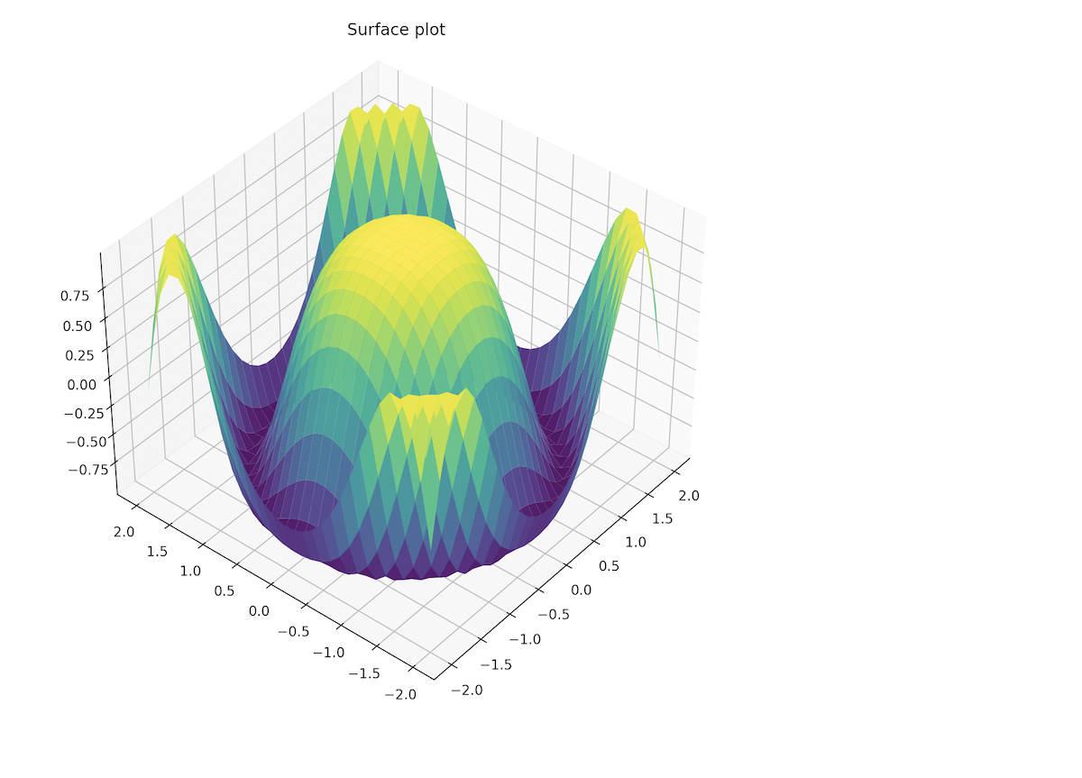
• Example 2, using Array, and Cos function to make a Surface plot.
  • Demo img
  • Code
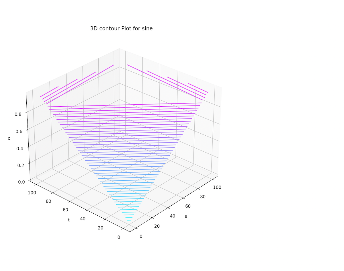
• Example 3, using Loops, List, and Sin function to make the contour plot.
  • Demo img
  • Code

Happy hacking!